viz, gpu, python - 2024-02-23

Rendering thick lines with dashes

Rendering lines on the GPU is notoriously non-trivial. Especially if you want special features like dashing, or have high standards like proper blending of semi-transparent lines. In this post I explain how we render lines in pygfx.

3D cubes with dashed lines

Introduction

In pygfx we have a line implementation that ticks a lot of boxes. Since the logic can be rather complex, this post serves as a more readable documentation, for those who want/need to maintain it. Plus it can be a useful to people who want to render lines themselves.

I don't go much into the details of shader code. The purpose of this document is to explain what the shader does in higher level terms. Please read the shader for the gory details.

In order to keep the bird's eye view, I'll refer to tricks that I posted separately in triangle tricks. You may want to read that first.

Setting off

For starters, we don't use vertex buffers. Instead we simply invoke the vertex shader six times for each point on the line, and sample the necessary data from storage buffers. This is trick 101. Because we use the triangle_strip topology, we have a total of 6 faces to work with. Two faces are used for the rectangular segment in between the points, leaving 4 faces to connect the segments (with a join).

Definitions

node: the positions that define the line. In other contexts these may be called vertices or points.
vertex: the "virtual vertices" generated in the vertex shader, in order to create a thick line with nice joins and caps.
segment: the rectangular piece of the line between two consecutive nodes.
join: the piece of the line to connect two segments. There are a few different shapes that can be applied.
broken join: joins with too sharp corners are rendered as two separate segments with caps.
cap: the beginning/end of the line and dashes. It typically extends a bit beyond the node (or dash end). There are multiple cap shapes.
stroke: when dashing is enabled, the stoke represents the "on" piece. This is the visible piece to which caps are added. Can go over a join, i.e. is not always straight.

Vertex placement

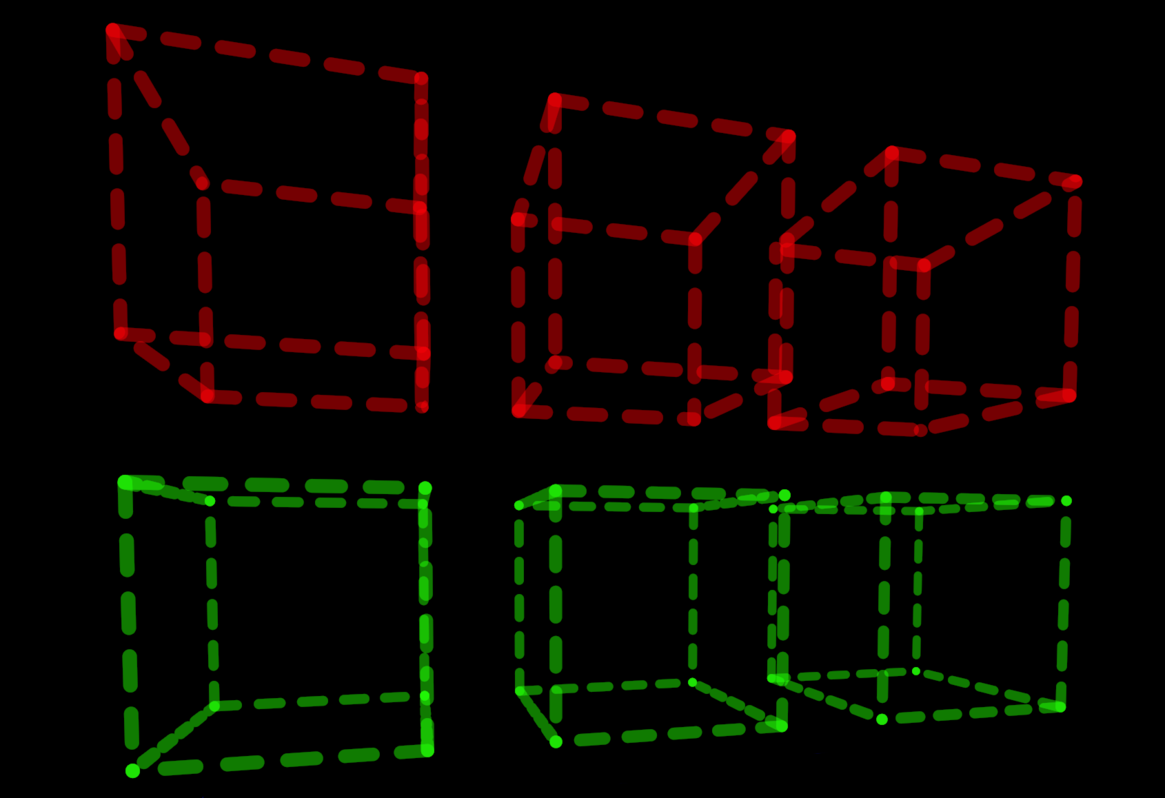
The six (virtual) vertices calculated in the vertex shader depend on the configuration. There are different configurations for caps, joins, and broken joins.

Cap

The very first and last node of a line are ends, and we draw caps on these instead. This also applies for line-pieces that are cut using a nan value. Since we only need 2 faces, the first/last vertices are placed in the first/last position respectively, leading to degenerate triangles (trick 7a).

The vertices that represent the segment egde (5 and 6 left, 1 and 2 right), are placed on both sides of the node, orthogonal to the line. The attached quad extends half the line width beyond the start/end of the line.

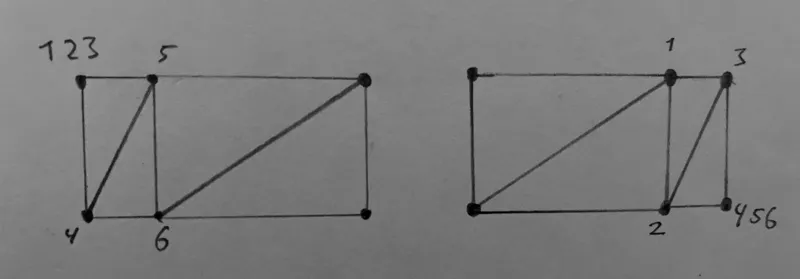
Join

In most cases, the segments on both side of a node are connected with a nice join. One can see how it actually consists of just two faces; the other two are degenerate. It also shows how vertex 3 and 4 are always placed in the outer corner. This makes that triangles 123 and 456 are independent (don't share a vertex), which is advantage later on. It also means that (depending on the direction of the corner) one of these triangles is inside-out, so we cannot use culling (trick 7b).) to discard faces.

Compared to the cap configuration, the segment does not extend up to the node. The vertices that represent the edge of the segment are inset, such that the segments touch exactly at the corner (26 left and 15 right). The opposing vertices (1 and 5 left, 2 and 6 right) are inset equally, to keep the segment square. Insetting the outer corner vertices is convenient/necessary for interpolating values cleanly over the join (as for e.g. dashing), but is otherwise not necessary.

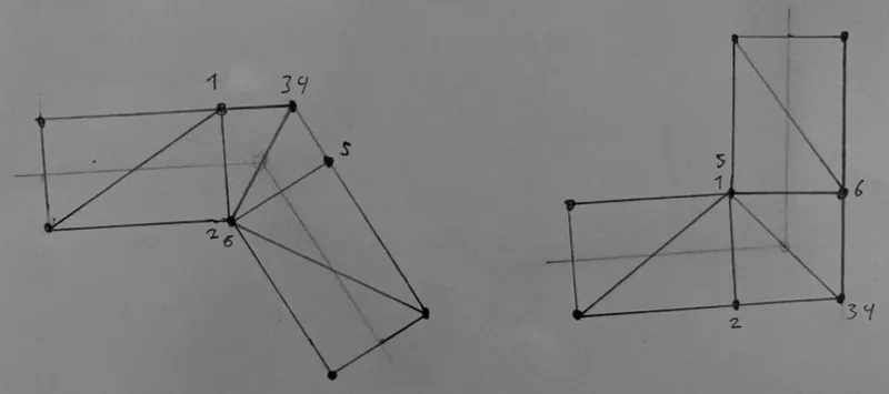
Broken join

The above configuration is restricted: the inset cannot go beyond half the distance between the nodes. If it would, we select the broken join configuration. Note that whether a join is broken or continuous thus depends on the angle between the segments, the line width, and the distance between the nodes.

A broken join consists of two segments with caps. We don't have enough vertices to use quads for the caps, so we use triangles instead. These extend a certain factor times the line width beyond the segment's edge. Round caps may have a very minor dent because of this. To properly separate the two caps, we drop the faces 234 and 345. We select these with trick 5b and then discard those fragments (trick 7c).

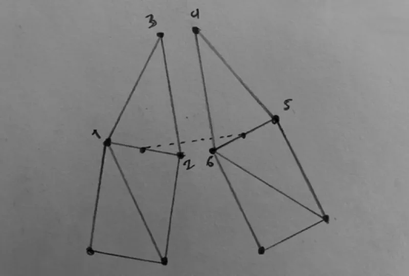
In reality, the end-point of both line pieces are in the same position, but for clarity they are drawn separately (see the stippled line).

The segment coordinate

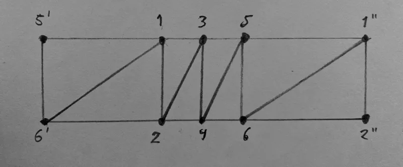
One important varying passed from the vertex to the fragment shader is the segment_coord. It represents the vector from the segment's centerline, and is used to sample the shapes of the caps and joins, and to perform antialiasing of the edges. Below is an illustration of its value for a piece of line that includes a cap, a join and (half of) a broken join.

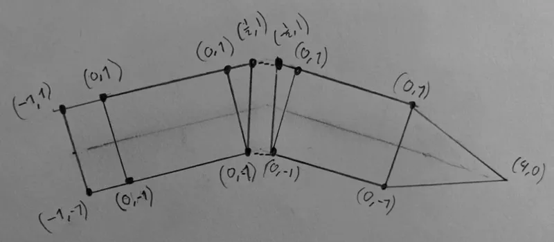
The coordinates apply to the segment, so the first triangle in a join has coordinates that apply to the segment of the left, and the second triangle in a join applies to the segment on the right. This is possible/easy because we can pass a different segment coordinate for vertex 3 and 4 (the advantage we mentioned earlier).

In the vertex shader, the segment_coord can be used to calculate the vertex position, by rotating it with the segment's angle and then using it as on offset for the node's position. Two birds with one stone!

In the fragment shader, this is all we need to handle caps. For joins, things are a bit more complicated.

The join coordinate

The way that the segment_coord is defined above won't allow us to parametrise a join just yet. We need a coordinate that describes the upper white square shown below (left).

This is one of the purposes of the join_coord. All vertices have this value set to 0.0, except vertex 3 and 4, which have a value of 1 and -1, respectively, when in a join. This results in a linear coordinate that - for each of the two faces in the join - goes from the segment's edge towards the corner. The isolines are shown in the left image below (trick 3). .

The join_coord can also be used to identify the faces that belong to the join (trick 5a). That way we can e.g. distinguish between cap and join shapes.

Inside a join, the join_coord can now be used to offset the segment_coord, so that the coordinate is centred around the line's node (the pivot point of the attached segments).

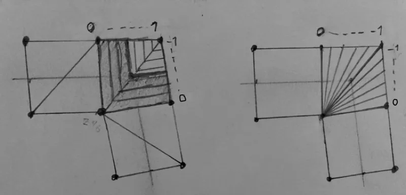
For interpolating values over a join, e.g. for per-vertex colors, or the cumulative distance in dashing, we also need a fan-shaped coordinate (join_coord_fan) to move the dashes around the corner. We calculate this by dividing the join_coord by a varying that is 1.0 for vertices in the outer corner (trick 4), resulting in isolines as shown in the above right image.

Joins and caps

In the fragment shader, the segment_coord is scaled with the line thickness, and expressed in physical coordinates, making it easy to work with.

It is then converted to a dist_to_stroke, the distance to the stroke's edge. Negative values mean that the fragment is inside the stroke. Positive means outside. Notice the resemblence with a scalar distance field.

The different joins and caps are implemented by different methods to calculate the dist_to_stroke. E.g. for round joins and caps, we can simply take the length of the segment_coord and discard fragments that are larger than half the line width.

Antialiasing

To perform antialiasing we define an edge, about 1 physical pixel wide, where the boundary of the stroke is. The dist_to_stroke value is a good measure for the coverage of that fragment, which is translated to an alpha value. This alpha value is squared, which is a pragmatic trick to prevent aa lines from looking thinner than they are.

To account for the boundary, the vertex coords are adjusted in the vertex shader as well, making the whole line just a wee bit wider.

Dashing

To implement dashing, we need extra work, which I explain in this section.

What we already took care of

The design outlined above was created with dashing in mind. In other words, if dashing is not needed, some things could be done different, possibly simpler.

In the design we took care not to have any overlap. One reason is that this avoids artifacts for semitransparent lines, but it's also a prerequisite for clean dashing.

Another point is that our segments are always rectangular; the vertices at the outer corner are inset by the same amount as the vertices at the inner corner. By doing this, we can also offset the cumulative distance (we'll get to that) on both sides of the join, so that we have something to work with to move dashes over the join.

Cumulative distance

One distinctive problem with drawing dashes, is the need for a cumulative distance to be known for each node on the line. Calculating this distance does not parallelize well. We opted to do this calculation on the CPU, just before each draw.

There are three flavours to distinguish between. One can calculate the distance in model space (the same space that the node positions are in), world space (the space of the scene), or in screen space. This matters especially in 3D applications: if a line points somewhat away from the camera, are the dashes closer together or not? As one zooms out, do the dashes stay the same size on screen? We let the user decide with a property on the line material.

Vertex shader

Once calculated, the cumulative distance is loaded into a GPU buffer, so we can load the value in the vertex shader. For each vertex, we produce two values, the cumdist_node represents the actual value at the node, and the cumdist_vertex represents the value at the vertex. This value is different from cumdist_node in the displaced vertices in a join, and the outset vertices in caps (including those in broken joins).

Fragment shader

In the fragment shader we use join_coord and join_coord_fan (depending on wheter it's a join) to interpolate between the two cumdist values, resulting in a smooth continuous value.

Note that this logic (passing the value over two-fold so it can be smoothly interpolated in the shader) can also be applied to other values, such as texture coordinates and per-vertex colors.

Once you have the cumulative distance, it's just a bit of math with a well-placed modulo operator to obtain the distance to the nearest dash stroke. This distance can be converted to a vector, using the segment_coord_p.y as it's y value. Then it can be converted to a "secondary" dist_to_stroke value. The final dist_to_stroke is the maximum of both.

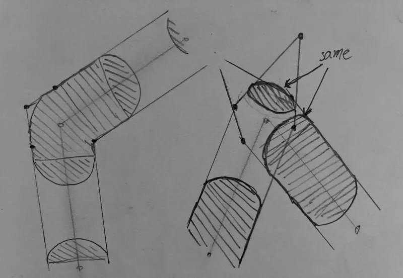
For broken joins, the two caps represent an area of duplicate cumulative distance. As illustrated in the right of the above image, this can result in dash-starts and dash-ends from being shown twice. To avoid this, we can use some logic that basically does this: if we are in the cap (of a broken join), and if the current dash would not be drawn in the segment attached to this cap, we don't draw it here either.

Conclusion

This concludes my high-level explanation of the thick-line shader in pygfx. Feel free to reach out for questions; I am happy to update this post to make it more clear.